A simple rule to identify if rare crimes have spiked
If you on average had 0.8 robberies in a month (so in between 9 and 10 per year), and you happened to have a month with 3 robberies, is that weird?
Part of being a crime analyst is monitoring temporal crime patterns – when you see a weird blip, you then go and do further analysis. For increases it may be you go and examine those cases more closely, to see if there is a serial offender that is causing the uptick. For decreases, you may do analysis to see if it is due to reporting issues, or some other event that is causing the crime occurrences to decrease.
If you are not careful though, you may be chasing the noise with what you think are significant increases, but are ups and downs in crime stats that can occur just by chance. For very rare events, especially if you are an analyst in a small jurisdiction, the above scenario is quite regular. To determine whether 3 is a weird spike, I am a big proponent of using the Poisson distribution to answer that question. So it ends up being that the probability of observing a month with 3 robberies, with a historical rate of 0.8 per month according to the Poisson distribution, is almost 4%.
The below table shows for a particular count in a month, the probability of observing that given a mean of 0.8 robberies per month. So you should have months with 0 robberies just under 45% of the time, and months with 1 robbery around 36% of the time, etc.
| Count | Percent |
|---|---|
| 0 | 44.9% |
| 1 | 35.9% |
| 2 | 14.4% |
| 3 | 3.8% |
| 4 | 0.8% |
| 5 | 0.1% |
| 6 | 0.0% |
To me, I would not flag 3 robberies as weird. It ends up being the expected number of 3 robbery months per year is almost 0.5 (so you would expect one month with 3 robberies about once every other year). I tend to only flag things that are closer to 1/100 to 1/1000 rare events. The reason for this is that as an analyst, you are not just monitoring robberies, you are monitoring at least a dozen (if not more) other temporal patterns.
Here this would result in needing 5+ robberies in a month to meet the less than 1/100 event criteria, or 6+ in a month to meet the 1/1000 criteria. It depends on how much time you have and how severe the crime is whether you want to set the threshold to 1/100 rare events or 1/1000 rare events.
Creating the Distribution In Excel
How did I calculate the above numbers? You can do this analysis quite easily in Excel. First, Create a table of the Counts (here in the first column) you want to examine. Then, in a place off of your table, place a cell with the mean number per month. Then in B2, you would use the formula =POISSON.DIST(A2,$F$1,TRUE). This gets you the probability of observing the counts in the A column given the mean in cell F1. You use the $ type cell reference to ensure later when we drag our formula to other values, it always references the F1 cell and does not change.
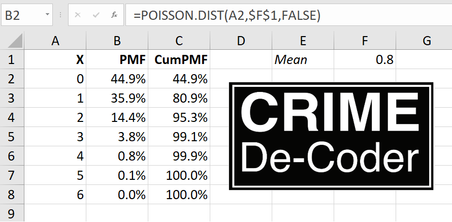
Now, like I said above, you would want to flag at 5+ or 6+ in this scenario, which means “5 or more” or “6 or more”. To get that threshold, you would want to calculate the cumulative percentage. So once you add up the probabilities for 0 through 4 counts, at that point we are above our 1/100 threshold (or a cumulative probability of over 0.99). To get the cumulative probability estimate, you can use the same formula, but change TRUE to FALSE.
And then you can drag your formulas down to fill in your table. If you update the mean cell, it will auto-update all of the calculations. You can download the spreadsheet here to check out the calculations.
Creating the distribution in R and Python
One of the reasons I like coding is that once you get the hang of it, it can be much simpler/faster than doing even ad-hoc data analysis tasks in Excel. Here I give examples of doing this analysis in R and python. R has all the necessary libraries to conduct this analysis by default, with the main function of interest dpois.
# R code to get density
mu <- 0.8
x <- 0:6
probs <- dpois(x,mu)
cumprob <- cumsum(probs)
res <- cbind(x,probs*100,cumprob*100)
print(round(res,1))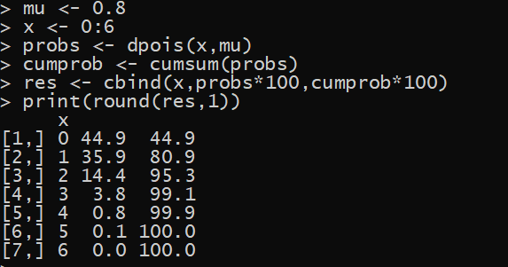
In Python it is slightly more work, as you need to have installed the scipy library (which if you use the Anaconda distribution of python it will be installed by default).
# Python code
from scipy.stats import poisson
mu = 0.8
x = list(range(7))
probs = poisson.pmf(x,mu)
cumprob = probs.cumsum()
for i,p,c in zip(x,probs,cumprob):
    print(f'{i} {p*100:.1f}% {c*100:.1f}%')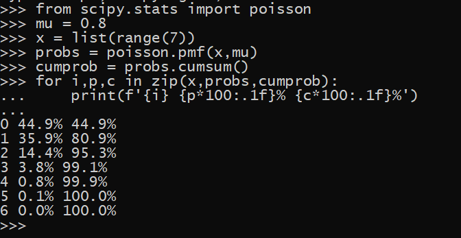
For those who are R fans, check out my ptools R package for other techniques to analysis count data. For those interested in python, check out my in progress book, Data Science for Crime Analysis with Python. Plan to have this out by next month, so this is close to the last chance to snag an early cheaper copy.
Upcoming Webinar
If you find this post interesting, with the Carolina Crime Analysis Association I am hosting a webinar on Monitoring Temporal Crime Trends.

I will go over this example, as well as a few others, in how I monitored temporal crime trends when I was a crime analyst.
You can sign up here, free for CCAA members and $10 for others, to view the webinar.
Excel Extra: Simulating Poisson Variates
One convenient way to understand how different data behaves is to conduct a simulation. If you want to do this in Excel for Poisson data, you cannot do this directly. You can however use a binomial approximation to the Poisson distribution to get quite close. The second sheet in the Excel document I shared has an example of doing this. To get random Poisson observations given a particular mean, you can use =BINOM.INV(50000,mean/50000,RAND()), where you fill in mean with the mean value reference.
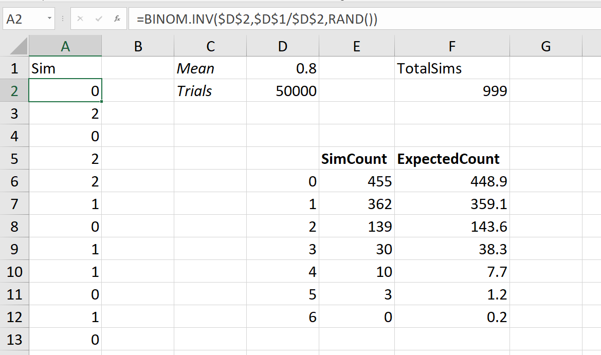
This can be convenient to check out the behavior of different methods to monitor crime patterns, e.g. pick a method, and then simulate data to see how your method does. If you want help in formulating different strategies to monitor and respond to crime, feel free to get in touch with CRIME De-Coder.