Confidence in Classification using LLMS

Confidence in Classification using LLMs and Conformal Sets

One of the common use cases for large language models is classifying text. Imagine you were monitoring a chat room for explicit language. You can tell the LLM, “Does this chat message have explicit language, return either True or False {message}”.

This is one of the benefits of LLMs vs traditional machine learning models. You did not have to train the model to specifically accomplish this task, it will generally do a good job of classifying across many categories and types of text.

In practice though, data scientists often not only want to know the category the model classified the text into, but the confidence in the classification. For the example monitoring for explicit language, you probably want to accept more false positives, but capture a higher proportion of the actual explicit messages. In different situations, you may want to control false positives.

In my book, LLMs for Mortals, one of the examples I discuss is examining log probabilities to get confidence in the classification. This example snippet from the book shows classifying whether a narrative involves a shooting.

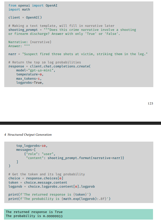
You can have the model not only return True or False tokens, you can also have certain models return the log probabilities that it chooses either of those tokens. You can see in this example it says the probability is 0.99999933 that the narrative contains the shooting.

What is that value exactly? It is the probability of the “True” token given the prior tokens. It is not a correct probability for our actual classification task. In other words, the probability is not calibrated. It is calibrated to generate tokens, not for our arbitrary task.

Because of this, it is hard to know where to set the threshold to classify a narrative as True or False. Even if True is returns a probability of over 0.999, you may want to classify that as False if you want to control false positives. Or the obverse, if it returns False, but the probability is 0.9, in some scenarios you may want to classify that as True.¹

For real systems, we are often interested in either recall, e.g. recovering 95% of the True cases, or controlling false positives, e.g. limit false positives to 1/10. These probabilities from the LLMs will not let you know that directly, but one way to figure it out is via conformal inference (example setting recall, example setting false positive rate).

To illustrate this, I use data from the Jigsaw toxic comment classification Kaggle competition. Here I illustrate classifying obscene comments from the competition. This is a useful benchmark as it has a large number of true samples to show against.

So what I do is batch process toxic classifications using gpt-4o-mini, and return the log probabilities. Here is the prompt, which not shown includes 30 k-shot examples of 10 obscene, 10 no toxic language, and 10 examples of other toxic label categories.

{k-shot-examples}

You are classifying online comments for toxic speech. 
Here we are identifying obscene comments. These include vulgar commentary
and profanity. Here are examples of comments and the expected binary classification:

{pos_txt}

I am now going to present a new comment. Return True if the comment is obscene, otherwise
return False. Only return True or False.

Example:

I then batch process a conformal sample of 3000 cases, and a total out of sample test sample of 50,000 records. The conformal sample I intentionally sample 1000 cases of obscene comments, 1000 cases of comments with no toxicity, and 1000 cases of comments with other toxic text (but are not classified as obscene). You can find code to replicate here on github. This just shows the end result analysis, which I saved the resulting classifications and log probabilities into 'MetricTestSamp.csv.zip' for the test sample of 50,000 records, and 'MetricConfSamp.csv.zip' for the conformal sample of 3000 cases.

First I load in the data with the classifications and the probabilities in the conformal sample and the test sample of cases.

# python code to set the conformal metrics
from binary_plots import *
from conformal_fp import ConfSet # conformal thresholds
import pandas as pd

test_sample = pd.read_csv('MetricTestSamp.csv.zip')
conf_sample = pd.read_csv('MetricConfSamp.csv.zip')
print(conf_sample.shape)
print(conf_sample.head())
print(conf_sample.tail())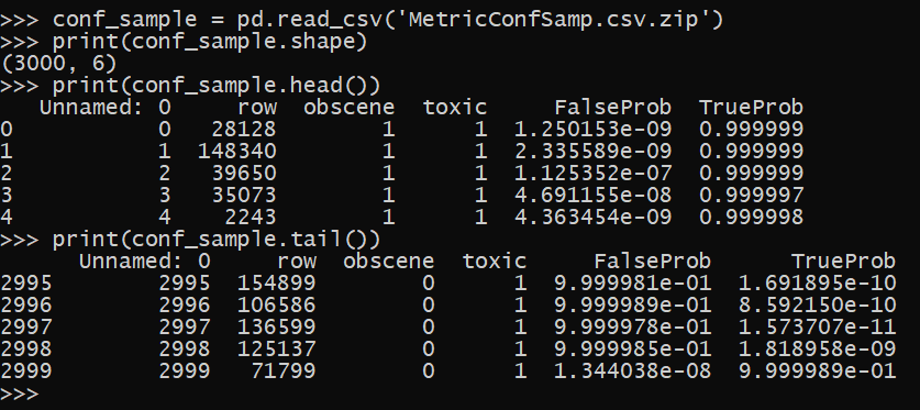

You can see the same as the example in the book, the probabilities tend to be highly clustered around near 0 and near 1 (so the model is over confident). If we examine the calibration though, the model has more false positives at very low probabilities and more false negatives at very high probabilities than you would expect with a well calibrated model.

# Examing the calibration
cal_res = cal_data('TrueProb', 'obscene', conf_sample,bins=10)
print(cal_res.to_markdown(index=False)) # this is actually not as bad as I thought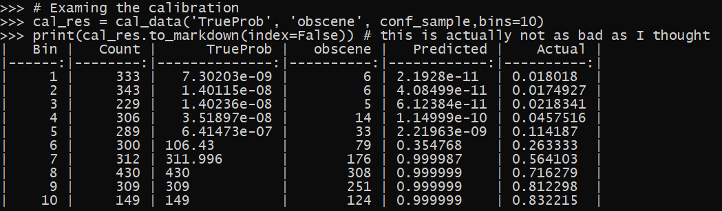

So here I use my conformal class (see the prior blog posts), passing in the predicted probabilities and the true outcomes in the conformal sample. Then I ask “what is the threshold needed to get 95% recall with this data”.

# Conformal method, true and probability
ct = ConfSet(conf_sample['obscene'],conf_sample['TrueProb'])

# If I want 95% recall, where is the threshold
rec95 = ct.Cover1(95)
print(rec95) # can see this is a very low value!

# And it is close to correct
oos_cov1 = (test_sample.loc[test_sample['obscene'] == 1,'TrueProb'] > rec95).mean()
print(oos_cov1)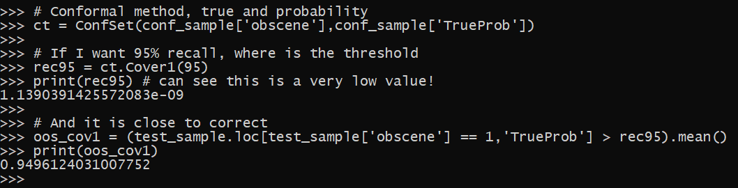

The probability ends up being very tiny, you want to set the threshold at 1.1390391425572083e-09! That is a probability with eight zeroes in front of it. You can see though in the example, this is what is necessary to get 95% recall. In practice you would have the model

One of the cool things about this, you don’t even need to know the actual distribution of obscene texts in the population. You can just sample obscene texts, get the distribution of their probabilities, and then look at the quantile to get this threshold.²

What if you want to control the false positive rate? To do that, we need to set the distribution of true positives you expect to see in the data. But otherwise, I have methods given a particular threshold, what do you expect the precision to be. Precision is if I classify 100 texts as obscene, what proportion are actually obscene (so 1 - precision is the false positive rate).

So here I set the threshold to 0.999999, and see what my expected precision is going to be.

# Need to set the overall proportion in the not sampled data
ct.SetProp(0.05)

thresh = 0.999999
c0, c1, prec = ct.PCover(thresh)
print(prec) # the precision is still not that high, only 72%

oos_prec = test_sample.loc[test_sample['TrueProb'] > thresh,'obscene'].mean()
print(oos_prec) # actual precision is somewhat higher than expected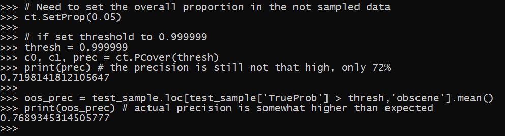

The estimated precision is 72%, and in our out of sample data the actual precision is under 77%. With this sample, I cannot estimate a threshold needed to say keep the precision at 99%. It would require classifying a large sample in the conformal sample, and in practice it may never be accurate enough to get that precise of an estimate with the general LLM model.

But at least with this method, you can get an estimate of the approximate number of false positives you expect if going into production.

This example for True/False can ultimately be extended for other classifications, or when extracting multiple elements from text. I suggest you check out my book, LLMs for Mortals (available as either an epub or paperback) for an entire chapter discussing extracting out structured information from text or documents.

Instead of looking at log probabilities, some authors just simply ask the LLM to return a probability value. This is generally not valid, but you could technically use the same conformal approach I am showing on those probabilities the model returns.↩︎
If you have small samples, you may want to use the method in this blog and not the actual quantiles in the data, especially when using quantiles at the more extremes of the data.↩︎